Contents
AirQuant Quickstart (Clinical Airways)
A quickstart tutorial to get going with AirQuant's functionality with example data!
tic
% You may need to run `AirQuantAddPath` before running this script to
% configure MATLAB to run AirQuant.
AirQuantDir = AirQuantAddPath();
See <a href = "https://airquant.readthedocs.io/">AirQuant Documentation</a> for help.
Download Data
First download the data!
dataname='chestct';
AQdownload_data(dataname);
See <a href = "https://airquant.readthedocs.io/">AirQuant Documentation</a> for help.
Downloading AirQuant dataset, "chestct" of 257 MB. This may take a while depending on your connection.
This case is from an opensource dataset, please see AirQuant readme for credits.
Load data
get data from nifti images into arrays and header variables.
% get CT, segmentation and skeleton images of the case
CT_name = [dataname, '_source.nii.gz'];
seg_name = [dataname, '_airway.nii.gz'];
skel_name = [dataname, '_airway_PTKskel.nii.gz'];

% Load data into relevant formations from nifti images.
% Load the source CT metadata information
meta = niftiinfo(CT_name);
% Load CT data as double
source = double(niftiread(meta));

% Load Airway segmentation and its skeleton as logicals
seg = logical(niftiread(seg_name));
skel = logical(niftiread(skel_name));
Make AirQuant object of data
There are lots of options here, be sure to check the documentation. This will process the skeleton of our image into its components for the AirQuant framework. Is the major step where the airway tree is broken down into its constituent branches. Splines are fitted to each branch, making the backbone of our analysis.
AQnet = ClinicalAirways(skel, source=source, header=meta, seg=seg, fillholes=1, largestCC=1, plane_sample_sz=0.5, spline_sample_sz=0.5);
% note: if you are running this in a live matlab script then the progress bar
% will not function properly.

% ClinicalAirways class has its own method for implementing automated lobe classification. We can call this to run on our image.
% The colour option can also be called for any visualisation method. Here
% it is called to show the lobes.
AQnet.ClassifyLungLobes();
Dimensions in physical units, usually millimetres.
Voxel dimensions = 0.63672     0.63672         0.5
Patch sampling size = 0.5
Spline sampling size = 0.5
Max plane size = 40
142 tubes found.
Tubes:SetGeneration :  100%  |██████████████████████████████████████| 142/142it [00:00:00<00:00:00, 6034.59 it/s]
Tubes:ComputeDirecti:  100%  |██████████████████████████████████████| 142/142it [00:00:00<00:00:00, 2301.65 it/s]
Tubes:ComputeChangeA:  100%  |██████████████████████████████████████| 142/142it [00:00:00<00:00:00, 7402.39 it/s]
Tubes:ComputeParentA:  100%  |██████████████████████████████████████| 142/142it [00:00:00<00:00:00, 7465.43 it/s]
Tubes:ComputeSibling:  100%  |██████████████████████████████████████| 142/142it [00:00:00<00:00:00, 6818.40 it/s]
Tubes:SetGeneration :  100%  |██████████████████████████████████████| 142/142it [00:00:00<00:00:00, 6249.72 it/s]
Basic visualisation
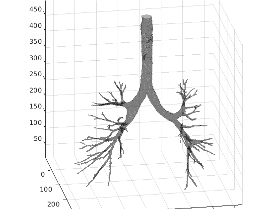
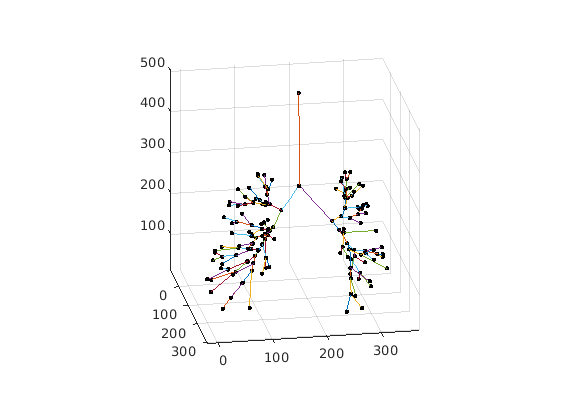
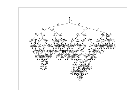
There are lots of visualisation options. Here we cover some basic options.
figure;
AQnet.Plot3D();

figure; AQnet.Plot3();
figure; AQnet.Plot();
% note that the edge labels correspond to the segment indicies
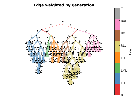
Advanced visualisation
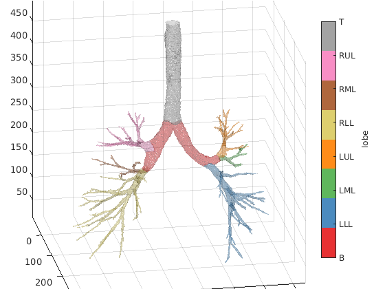
We can use the lobe region classifications to further enrich our visualisation. Checkout the documentation for more advanced visualision use cases.
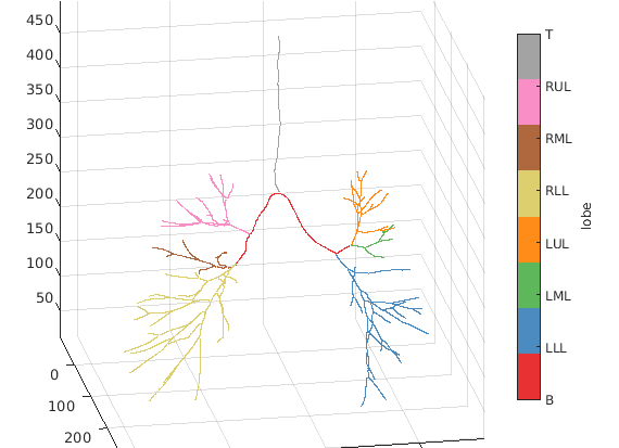
figure; AQnet.Plot(colour='lobe', weight='generation', weightfactor=10);
title('Edge weighted by generation')
figure; AQnet.Plot3D(colour='lobe');
% `Plot3D` can be resourse demanding on your specs. You maywant to
% skip it.
figure; AQnet.PlotSpline(colour='lobe');
Export values to csv
Finally we can export our values to a csv file for easy analysis in our next favourite package!
AQnet.ExportCSV('example.csv');
% print first 10 rows of example.csv
T = readtable('example.csv');
T(1:10,:)
toc
ans =

  10×15 table

    ID    children_1    children_2    children_3    generation    method    parent    region_lobe        region_name         stats_arclength    stats_change_deg    stats_euclength    stats_parent_deg    stats_sibling_deg    stats_tortuosity
    __    __________    __________    __________    __________    ______    ______    ___________    ____________________    _______________    ________________    _______________    ________________    _________________    ________________

     1         2             3           NaN            0          NaN       NaN        {'T'  }      {'Trachea'         }        109.42              16.708             106.45                 NaN                 NaN               1.0278
     2         4             5           NaN            1          NaN         1        {'B'  }      {'LeftMajor'       }        59.976              11.784             57.322              36.332              141.72               1.0463
     3         6             7           NaN            1          NaN         1        {'B'  }      {'RightMajor'      }        37.229              40.222             34.813              105.86              141.72               1.0694
     4         8             9           NaN            2          NaN         2        {'LLL'}      {0×0 char          }         13.42              61.068             12.467              93.493              121.23               1.0764
     5        10            11           NaN            2          NaN         2        {'B'  }      {'LeftIntermedius' }        12.758              31.189             12.367              28.605              121.23               1.0316
     6        12            13           NaN            2          NaN         3        {'B'  }      {'RightIntermedius'}         23.72              68.463             22.419              54.851              127.15                1.058
     7        14            15            16            2          NaN         3        {'RUL'}      {0×0 char          }        15.757              10.596             15.312              79.511              127.15                1.029
     8        17            18           NaN            3          NaN         4        {'LLL'}      {0×0 char          }        20.557              46.134             19.925               111.5              129.92               1.0317
     9        19            20            21            3          NaN         4        {'LLL'}      {0×0 char          }        9.7253              27.097             9.2612              22.602              129.92               1.0501
    10        22            23           NaN            3          NaN         5        {'LML'}      {0×0 char          }        16.521              14.084             16.446              57.132              44.191               1.0045

Elapsed time is 69.855670 seconds.