Contents
AirQuant FWHM (Clinical Airways)
This tutorial assumes you have run the quickstart tutorial and have built the `ClinicalAirways` object saved as `AQnet`.
Now that the backbone of the AirQuant analysis has been set up, we can work through subsequent steps of interpolating the source image for airway measurement. we opt to only demonstrate this on one airway, though in reality we want this to be done on every airway. We pick one airway id.
tic
% You may need to run `AirQuantAddPath` before running this script to
% configure MATLAB to run AirQuant.
AirQuantDir = AirQuantAddPath();
See <a href = "https://airquant.readthedocs.io/">AirQuant Documentation</a> for help.
Single airway/tube patch interpolation and FWHMesl
we can access any 'tube' (airway) by its index, this allows us to access the methods of tubes.
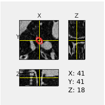
atube = AQnet.tubes(10);

% We run the method make the airway patch slices of this airway on the CT.
usegpu = 0;
atube.MakePatchSlices(AQnet.source, type='source', method='linear', gpu=usegpu);

% set up parameters of FWHMesl
% With our airway patches interpolated we now run the measurement of each patch. We a very straightforward method, FWHMesl.
num_rays = 60;
ray_interval = 0.2;
% segmentation interpolation is also required for the FWHMesl method
atube.MakePatchSlices(AQnet.seg, type='seg', method='linear', gpu=usegpu);
atube.Measure('AirwayFWHMesl', num_rays, ray_interval);

%   We can interactively visualise the CT image along the airway patches with its estimated ellipse fitting.
% (opens externally)
figure; atube.OrthoView();
Basic visualisation
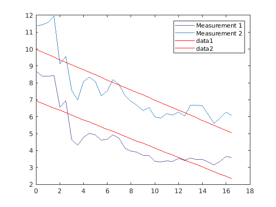
We can plot any measurement along the airway against its arc-length
figure; atube.plot(Y='diameters');
% though this is the default options for X and Y, we will be explicit.
Export individual airway/tube
atube.ExportCSV('example.csv');
% print first 10 rows of example.csv
T = readtable('example.csv');
T(1:10,:)
ans =

  10×8 table

    patchprop_parapoints    patchprop_arcpoints    patchprop_hydraulic_diameter_1    patchprop_hydraulic_diameter_2    diameters_1    diameters_2    areas_1    areas_2
    ____________________    ___________________    ______________________________    ______________________________    ___________    ___________    _______    _______

                0                     0                        4.1821                            5.5801                  8.6861         11.376       59.258     101.65
          0.51138                   0.5                        4.0957                            5.6672                     8.4         11.423       55.417     102.47
           1.0202                     1                         4.099                            5.7358                  8.3941         11.577        55.34     105.27
           1.5261                   1.5                        4.1442                            5.9386                  8.4346         11.961       55.876     112.36
            2.035                     2                        3.2137                            4.4179                  6.5737         9.1138       33.939     65.236
           2.5531                   2.5                        3.4288                            4.7814                  6.9293         9.5775       37.712     72.043
           3.0845                     3                         2.234                            3.7067                   4.633         7.5485       16.858     44.752
           3.6301                   3.5                        2.1077                             3.474                   4.328         6.9874       14.712     38.346
            4.184                     4                        2.3562                            4.0027                  4.7744         8.0743       17.903     51.203
           4.7337                   4.5                        2.4931                            4.1682                  5.0059         8.3534       19.681     54.804
process all airways to make patches
We can process all airways now. This can take somewhere between 1-4 hours to run. By default it will try to run on GPU if available which can speed things up. uncomment the lines below to run.
% AQnet.MakeTubePatches(method='linear', gpu=usegpu)
% AQnet.Measure('AirwayFWHMesl', num_rays, ray_interval);

% We can now visualise the characteristics derived from diameter measurements.
% figure; AQnet.Plot(colour='lobe', weight='meandiameter', weightfactor='10')

toc
Elapsed time is 23.171602 seconds.